Research

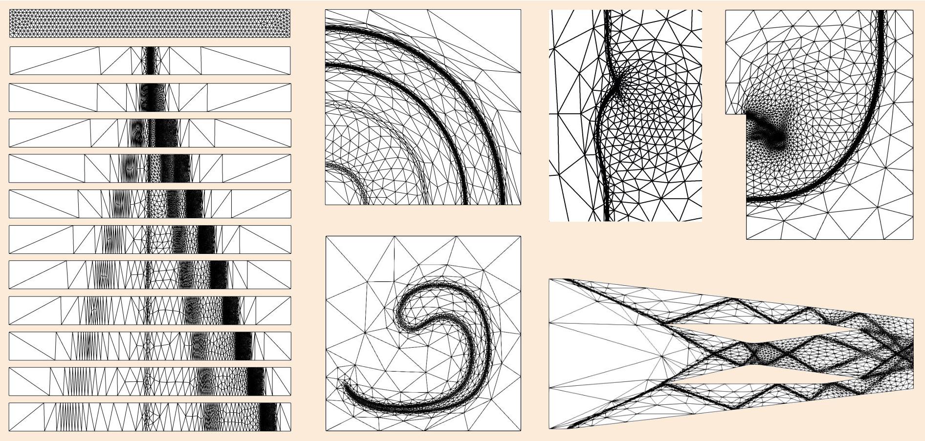
My research is concerned with the development of advanced numerical methods for time-dependent compressible flow problems. In particular, I work on adaptive discontinuous Galerkin methods, anisotropic mesh adaptation, and conservative solution transfer between non-matching meshes. The aim is to improve the robustness and efficiency of simulations involving complex transient flow phenomena. Selected numerical examples shown below illustrate the main ideas and capabilities of the developed approach so far.

Research Topics

• High-order numerical methods for compressible flow
• (Hybridized) discontinuous Galerkin methods
• Anisotropic mesh adaptation
• Conservative solution transfer between non-matching meshes
• Time-accurate simulation of transient flows
• Shock-dominated compressible flow problems

The selected examples below illustrate how these topics come together in representative numerical test cases and adaptive simulations.

Research Highlights

• Time-accurate adaptive HDG framework. Development of a time-accurate adaptive hybridized discontinuous Galerkin (HDG) framework for compressible flow problems, with particular emphasis on combining time-dependent simulations with anisotropic mesh adaptation.

• Conservative solution transfer. Development and implementation of a conservative solution transfer algorithm for non-matching meshes arising from anisotropic mesh adaptation, enabling reliable transfer of the numerical solution while preserving physical quantities over the computational domain.

• Application to challenging test cases. Application of the developed methods to representative time-dependent problems, with emphasis on the Euler equations, including cases with sharp gradients, discontinuities, and other complex evolving flow structures.

• Extension to three-dimensional tetrahedral meshes. Extension of the transfer methodology from two-dimensional settings to three-dimensional tetrahedral meshes, providing the basis for adaptive solution transfer in more realistic 3D simulations.

Representative Test Cases

The examples presented below are based on the Euler equations and illustrate representative applications of the developed adaptive HDG framework. Beyond the assessment of numerical accuracy, they are used to demonstrate the behaviour of the solver in combination with anisotropic mesh adaptation for transient problems. To support this process, a mesh prediction strategy based on a lower-order time integration method (Backward Euler) was developed for adaptive mesh refinement in time-dependent simulations. The general aim is to provide the solver with an initial mesh that is as simple and as easy to generate as possible, while allowing it to adapt both at the initial stage and throughout the simulation wherever increased resolution is required by the evolving flow field.

1) Shock-Vortex Interaction

2) Sod’s Shock Tube Problem

3) Explosion Problem

4) Shock Diffraction Problem

All examples in this section are based on the two-dimensional compressible Euler equations

\[\frac{\partial \mathbf{u}}{\partial t} + \frac{\partial \mathbf{f}_1(\mathbf{u})}{\partial x} + \frac{\partial \mathbf{f}_2(\mathbf{u})}{\partial y} = 0,\]

where $\mathbf{u} = \left[\, \rho, \,
\rho u, \,
\rho v, \,
E \, \right]^T$ is the vector of conservative variables, with density $\rho$, velocity components $u, v$, and total energy $E$ and

\[\mathbf{f}_1(\mathbf{u}) = \left[ \, \rho u, \, \rho u^2 + P, \, \rho u v, \, (E + P) u \, \right]^T\] \[\mathbf{f}_2(\mathbf{u}) = \left[ \, \rho v, \, \rho u v, \, \rho v^2 + P, \, (E + P) v \, \right]^T\]

are the flux vectors. The pressure $P$ is given by the ideal gas law

\[P = (\gamma - 1) \left( E - \frac{1}{2} \rho (u^2 + v^2) \right)\]

where $\gamma$ is the ratio of specific heats, taken to be $\gamma = 1.4$ in all examples.

Last update: 2026-07-22 12:55:28 +0000