Sod’s Shock Tube Problem

Related publication: Levý & May (2025)

This example considers the classical Sod shock tube problem for the Euler equations, extended here to a two-dimensional setting. The solution develops the characteristic three-wave structure of a Riemann problem, namely a rarefaction wave, a contact discontinuity, and a moving shock wave. As such, the problem provides a convenient test case for studying adaptive simulations in the presence of moving discontinuities.

In this case, the initial discontinuity is located at $x = 0.5$ and the solution evolves in the domain $[0,1] \times [-0.05,0.05]$ up to the final time $T = 0.25$. Initially, the discontinuous initial condition is projected onto a uniform coarse mesh used as the starting mesh for the solver.

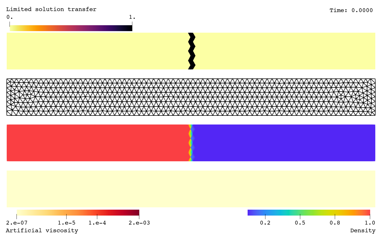
Initial condition for the Sod's shock tube problem on initial uniform coarse mesh with 1,200 elements. The upper panel shows discontinuity detection and the corresponding region where projection limiting is applied.

The initial projection then serves as input to the initial anisotropic mesh adaptation, which produces the first initially adapted mesh shown below. This mesh and the corresponding projected initial condition are then used as input for the first time step of the simulation.

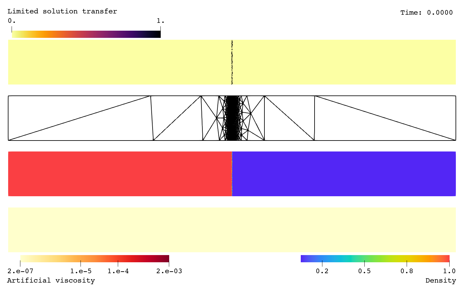
Initial condition for the Sod's shock tube problem on initially adapted anisotropic mesh with 1,000 elements.

In the present context, the main role of this example is to illustrate the importance of the mesh-predictor strategy for moving shocks. Since the dominant wave structures propagate through the domain, the mesh cannot be adapted reliably based only on the immediate numerical solution at hand. Instead, the predictor provides a mechanism for anticipating the near-future evolution of the solution and for constructing meshes that remain consistent with the flow features during the adaptation interval. In addition, it allows for larger adaptation intervals and thus reduces the frequency of remeshing.

The computation is performed with polynomial degree $p = 2$ and the Backward Euler method with $\mathrm{CFL}=1$ up to the final time $T = 0.25$. Starting from a uniform mesh of 1,200 elements, the adapted mesh is restricted to at most 1,000 elements. The resulting mesh evolution shows that the predictor-based strategy is able to follow the travelling discontinuities in a stable and physically consistent manner, while maintaining a low overall number of elements.

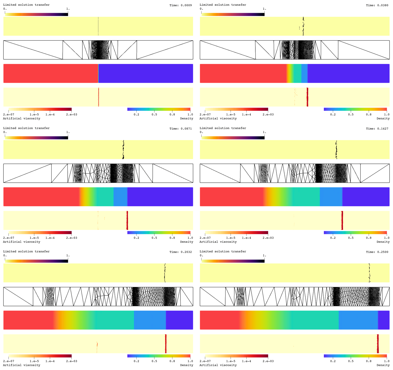
Simulation of the Sod shock tube problem using the mesh-predictor approach. The mesh is adapted every adaptation interval $\Delta t_A = 0.025$ based on the predictor solution, with a maximum of 1,000 elements. Resolution is concentrated near the shock wave, the contact discontinuity, and the rarefaction region, while smooth parts of the solution remain comparatively coarse.

The contour plot at the bottom of each figure shows the artificial viscosity field used to stabilize the solution in the presence of shocks. The viscosity is primarily activated near the shock wave, while remaining negligible in smooth regions of the flow.

Last update: 2026-07-22 12:55:28 +0000